Visualizing Point Clouds

Assuming you have a dataset of particles (e.g. dark matter particles in cosmological simulation, SPH-particles, etc.) and their coordinates, there are multiple ways to browse through them as a 3D point cloud.

# Using Paraview

The most interactive method is using Paraview. It can read many input formats, but for simplicity we are using CSV files with columns for X, Y and Z coordinates here.

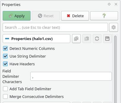
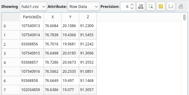
After opening the CSV with the right delimiter we get a SpreadSheetView displaying the data.

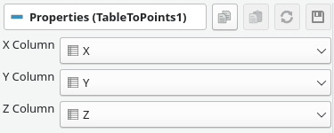
To now draw points for all particles, we go back to the default RenderView and select Filters -> Alphabetical -> Table to Points. First we need to assign the columns to the dimensions before clicking on “Apply”.

If you don’t see any points, check if you have focused the RenderView and the eye symbol in the Pipeline Browser is enabled. If the particles are not centered or very small (e.g. because of accidentally plotting the particle ID as a dimension before), one can open the “Adjust Camera” menu of the RenderView and select a Standard Viewpoint.

If your dataset has an additional column, you can color the points according to it by selecting it in the “Coloring” section. The used colormap can be edited to e.g. use logarithmic values.

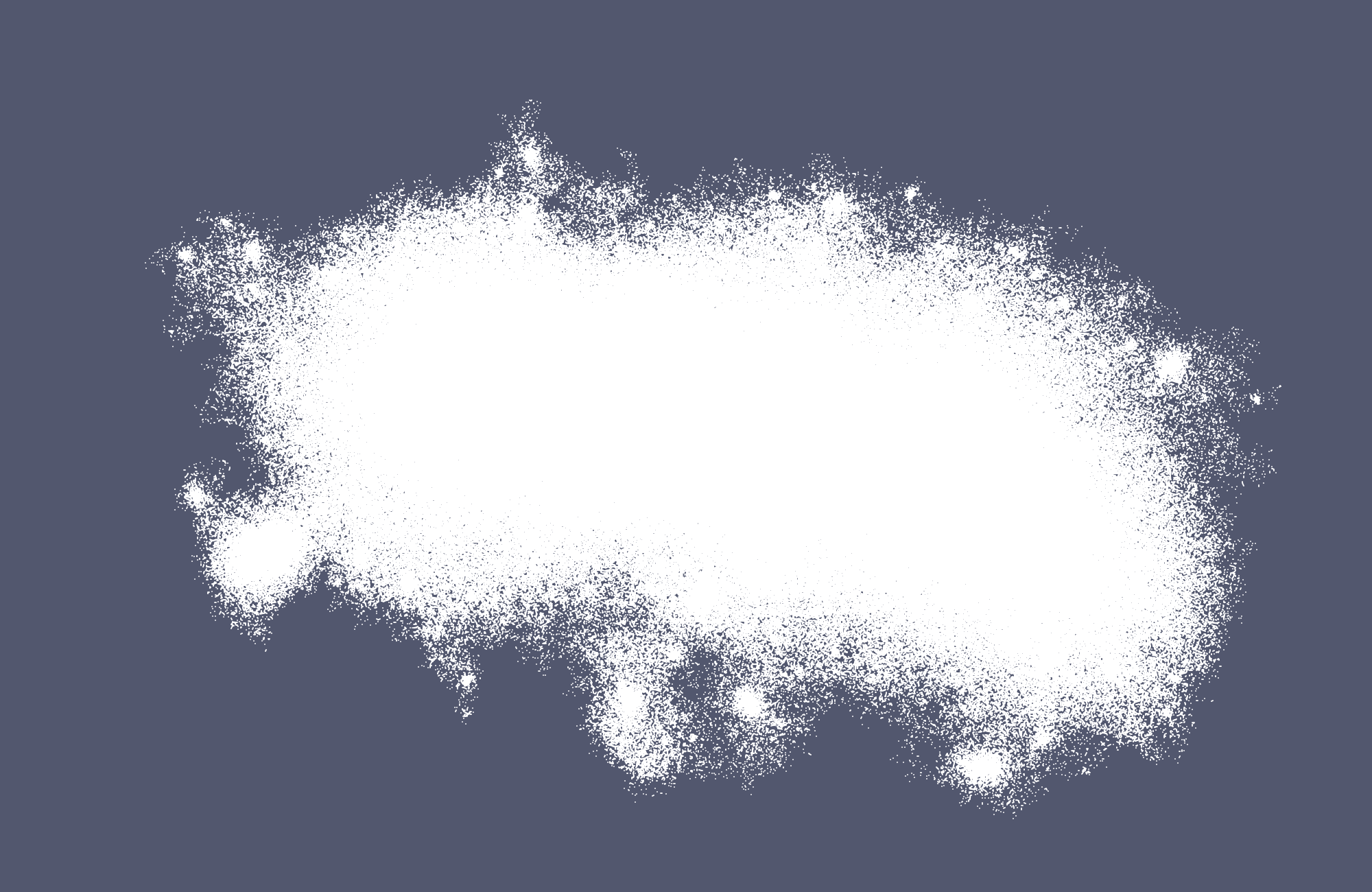
As a next step, reducing the opacity allows us to better see the distribution of the particle density. Depending on the number of particles a very low value can be used (e.g. 0.02 here for 2 million particles).

Still areas with high density are just white blobs and the level of detail depends on the zoom level as the size of the points is always the same.

One solution to this problem is to use Point Gaussians instead of points to represent every particle. For this select “Point Gaussian” from the “Representation” drop-down. In the new “Point Gaussian” you can then change the shader preset. While “Sphere” might work with a small amount of large masses, representing them as a “Gaussian Blur” works best for large amounts of particles.

If you see triangle-like structures, try changing the opacity. Once again we need to set the Gaussian Radius to a very low value until all details can be differentiated.

# In Python

While Paraview is very powerful, often it is useful to display a subset of data automatically during data analysis without needing to export and open the dataset every time. Therefore, it is useful to create the same visualisation in Python.

For this we are using vtk which Paraview is based on. As the Python VTK wrapper is not always very user-friendly, the best solution is pyvista, which abstracts many of these details away.

$ pip install pyvista

Let’s assume data is a numpy array with three columns corresponding to the position of the particles (similar to the output of np.random.random((10000, 3))).

Then we can initialize a pyvista Plotter like this:

from pyvista import Plotter

pl = Plotter()

Next we need to convert the data to a PointSet:

pdata = pyvista.PointSet(data)
# data[::, 0:3] if there are more than three columns

Then we can plot the data:

pl.add_mesh(
    pdata,
    point_size=1,
    style="points",
    opacity=0.1,
    color="white",
    # scalars=data[::, -1], # if we had a column with values
)
pl.enable_parallel_projection()

Instead of specifying style="points" explicitly, we could also use pl.add_points() directly. Once again point_size and opacity can be adapted to the dataset.

Finally, we can open the window using

pl.show()

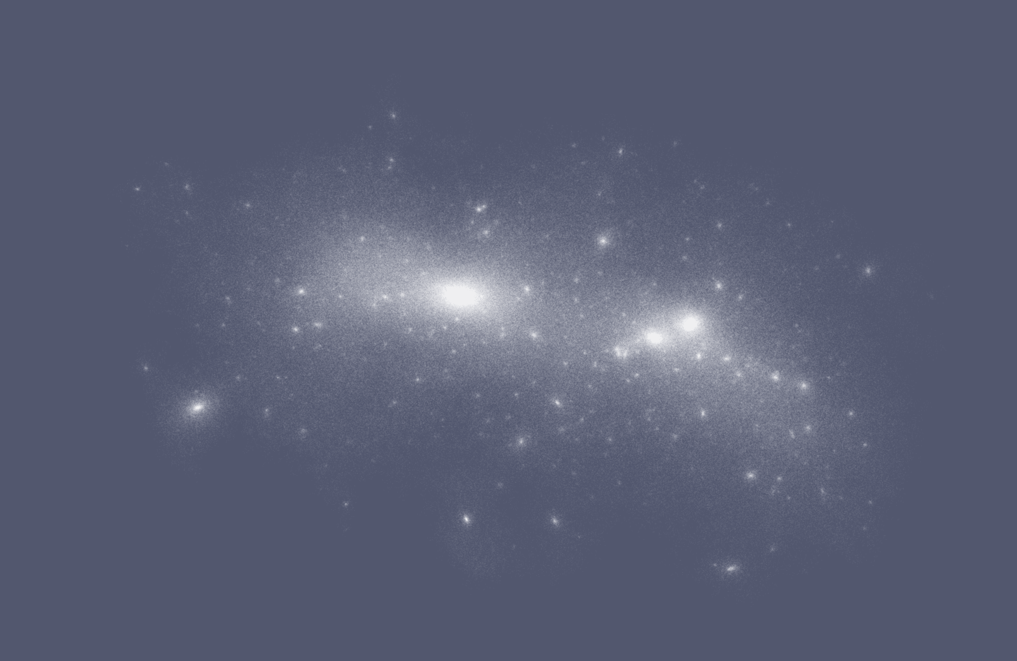
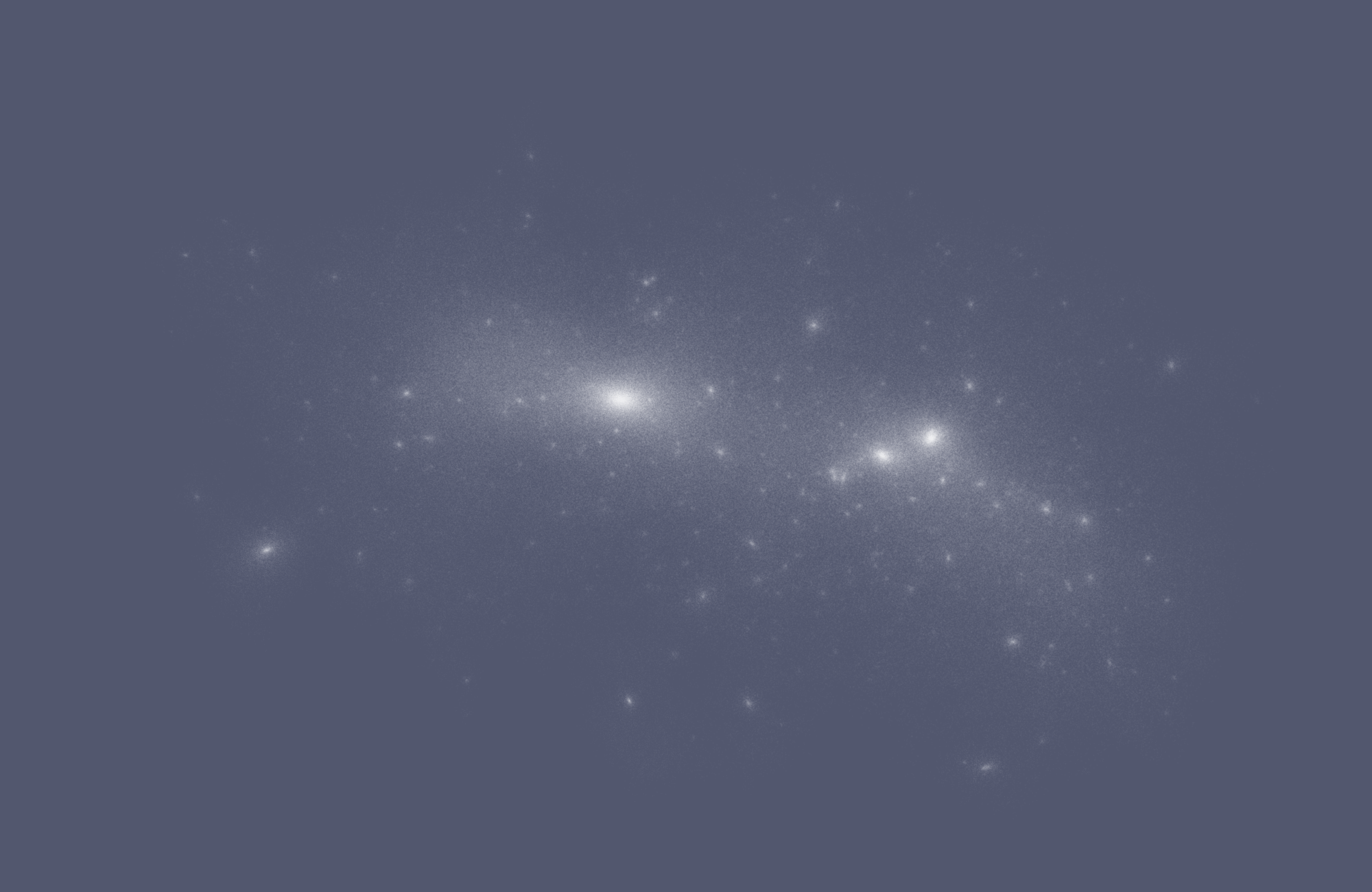
Unlike the paraview visualisation, here we for now only show each dataset as an individual dot. But just like the “Point Gaussians” setting in Paraview, we can change the visualisation to instead show every datapoint as a gaussian blur, thanks to the pyvista developers.

pl.add_mesh(
    pdata,
    point_size=0.2,
    style="points_gaussian",
    render_points_as_spheres=False,
    emissive=False,
    opacity=0.2,
    color="white",
)

https://docs.pyvista.org/version/stable/examples/02-plot/point-clouds.html

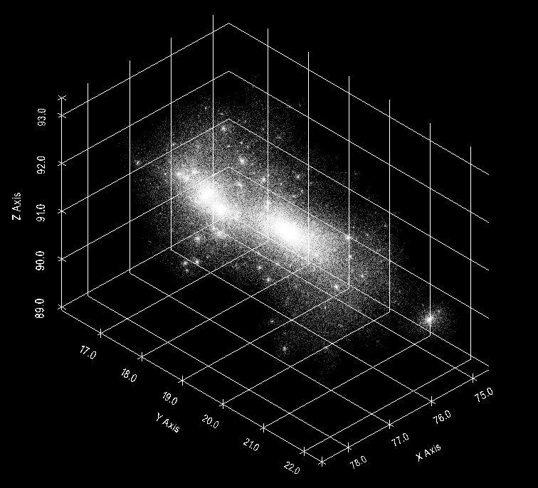
If we know the center of the object, we can manually specify it using

pl.set_focus((halo.X, halo.Y, halo.Z))

Also a grid can be added:

pl.show_grid()

And optionally the output can be rendered in 3d:

pl.enable_stereo_render()
# use one of the many SetStereoTypeTo*() functions
pl.ren_win.SetStereoTypeToSplitViewportHorizontal()
pl.ren_win.SetStereoTypeToAnaglyph()

If you prefer different mouse-controls where the negative z-axis always points down, you might want to enable terrain style:

pl.enable_terrain_style()

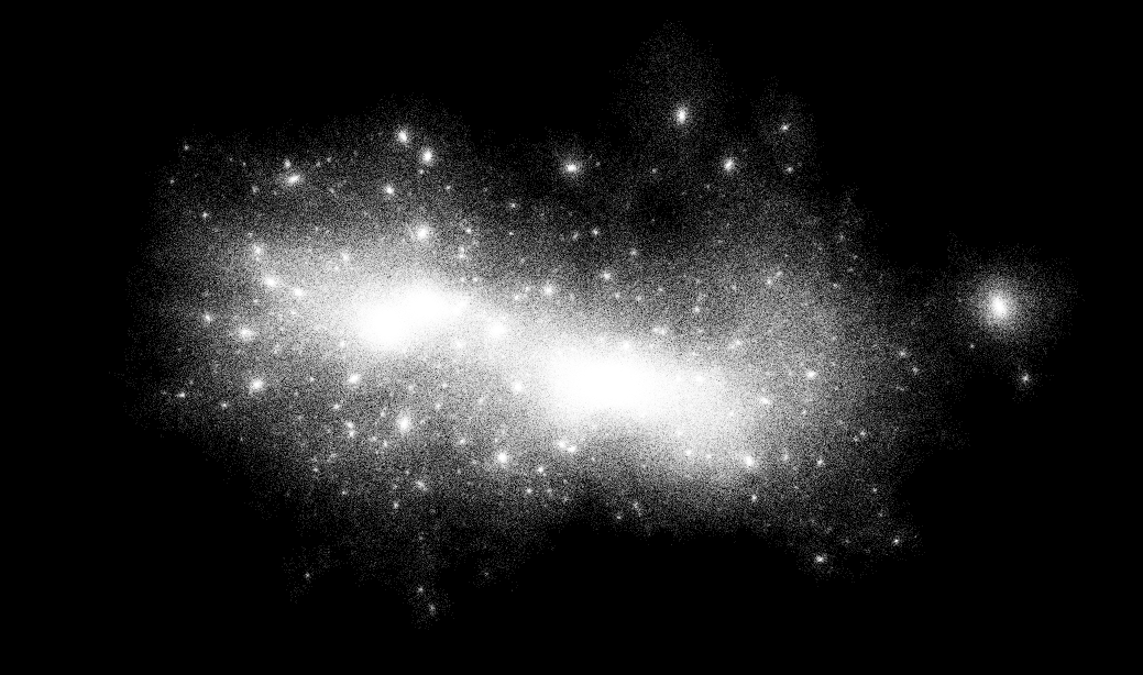
A regular graphics card should be able to display millions of points in real-time.

Even with 512^3 particles the visualisation is still very interactive:

# Videos in Python

While pyvista supports creating simple MP4 videos out of the box, we can also do more complex automation of screenshots and camera:

pl = Plotter(window_size=[800, 800])
pl.ren_win.OffScreenRenderingOn() #  optional, needed if the window_size is larger than the screen resolution
pl.show(auto_close=False, interactive=False)

# orbit around center
path = pl.generate_orbital_path(n_points=250, shift=150, factor=2, viewup=[0, 0, 1])
global_i = 0
for i, point in enumerate(path.points):
    pl.set_position(point, render=False)
    pl.set_focus(pl.center, render=False)
    pl.render()
    pl.screenshot(f"/tmp/images/test_{global_i:04d}.png")
    global_i += 1
start_pos = np.array(path.points[0])

# very simple zoom
end_pos = np.array([50, 50, 50])
diff_vec = end_pos - start_pos
for i in range(250):
    pl.set_position(start_pos + diff_vec * i / 250, render=False)
    pl.set_focus(end_pos, render=False)
    pl.render()
    pl.screenshot(f"/tmp/images/test_{global_i:04d}.png")
    global_i += 1
for i in range(125):
    pl.set_position(end_pos - diff_vec * i / 125, render=False)
    pl.set_focus(end_pos, render=False)
    pl.render()
    pl.screenshot(f"/tmp/images/test_{global_i:04d}.png")
    global_i += 1
pl.close()

Unfortunately a large amount of particles causes fine-grained “random” noise in the image which compresses extremly badly in videos.

# Bonus: Exporting Videos for Publication

Exporting Videos in Paraview and similar tools is rather easy, but the options are often quite limited and only support older formats and codecs. Therefore, the resulting videos can often be quite large and in low quality which is especially bad for point clouds where a lot of fine details can be lost in video compression.

Because of this it is often useful to export the video as a collection of (losslessly compressed) PNG files and encode the video yourself.

The following options are optimized for a high quality while still having a small file size, which means they can be slow to encode. But as most videos are rather short, this should not be that important. Also, the videos embedded in this page are compressed more to keep the loading time small while loosing only little quality.

# VP9

VP9 is a widely supported modern video codec.

For the best results a two-pass encoding is used with the first command saving a temporary file and the second command actually encoding the file.

$ ffmpeg -framerate 30 -i img.%04d.png -c:v libvpx-vp9 -pass 1 -crf 35 -b:v 5M -deadline good -cpu-used 0 -row-mt -tile-columns 3 -frame-parallel 1 -an -pix_fmt yuv420p -f webm -y /dev/null

$ ffmpeg -framerate 30 -i img.%04d.png -c:v libvpx-vp9 -pass 2 -crf 35 -b:v 5M -deadline good -cpu-used 0 -row-mt -tile-columns 3 -frame-parallel 1 -auto-alt-ref 1 -lag-in-frames 25 -pix_fmt yuv420p -f webm -y out.webm

Important options:

• -framerate: set to the amount of frames per second
• -i img.%04d.png: this assumes the images are called img.0001.png
• -crf 35: the Constant Rate Factor describing the quality of the output. It can be a value from 0 to 63 with lover values indicating a higher quality. In general recommended values range from 15 to 35, but for complex videos a higher value might be needed to not create huge files.
• -b:v 5M: Optionally, in addition to -crf one can also set a constraint on the maximum bitrate (so 5 Mbit/s here) to limit the file size.
• -pix_fmt yuv420p: chroma subsampling for compression and support in browsers
• -y: answer “yes” when asked to overwrite existing files
• out.webm use WebM as a container format for the output file

If the input is an existing video file instead of a list of images, replace -framerate 30 -i img.%04d.png with -i input.mp4.

Additional options:

• -an: remove an audio stream from the input video

More information about the options can be found here.

# MP4 (H.264)

Some browsers don’t support VP9 yet (most notably Safari), so a fallback to MP4 might be useful as it is supported on most devices:

Here, we also use a Constant Rate Factor (CRF) to specify the quality. It can go from 0 to 51 with a lower value indicating a higher quality. Values around 20 might be a good starting range.

$ ffmpeg -framerate 30 -i img.%04d.png -vcodec h264 -b:v 1M -strict -2 -pix_fmt yuv420p -preset veryslow -crf 20 -movflags +faststart -y out.mp4

# Display in browsers

You can use the <video> tag to embed videos in websites.

For gif-like looping videos:

<video autoplay loop muted controls playsinline>
    <source src="video.webm" type="video/webm; codecs=vp9">
    <source src="video.mp4" type="video/mp4">
</video>

For regular videos (only load the metadata/thumbnail until pressing play):

<video preload="metadata" muted controls playsinline>
    <source src="video.webm" type="video/webm; codecs=vp9">
    <source src="video.mp4" type="video/mp4">
</video>